Compare with chromVAR: Part I

Since we completely re-implemented the algorithm proposed in chromVAR in Python, we may want to confirm that these two packages can produce the similar, if not exactly same, results. So here we test them on a small example data from chromVAR.

Run chromVAR on example data

We first load the packages that we need

suppressMessages(library(chromVAR))
suppressMessages(library(Repitools))
suppressMessages(library(SummarizedExperiment))
suppressMessages(library(motifmatchr))
suppressMessages(library(Matrix))
suppressMessages(library(BiocParallel))
suppressMessages(library(BSgenome.Hsapiens.UCSC.hg19))
suppressMessages(library(JASPAR2020))
suppressMessages(library(TFBSTools))
set.seed(2017)

Let’s get the example count matrix

data(example_counts, package = "chromVAR")

We can check how the peaks look like:

df_peaks <- annoGR2DF(example_counts@rowRanges)
df_peaks$peak <- paste0(df_peaks$chr, "-", df_peaks$start, "-", df_peaks$end)
head(df_peaks)

A data.frame: 6 × 8

	chr	start	end	width	score	qval	name	peak
	<fct>	<int>	<int>	<int>	<int>	<dbl>	<chr>	<chr>
1	chr1	713933	714432	500	259	25.99629	GM_peak_6	chr1-713933-714432
2	chr1	856395	856894	500	82	8.21494	H1_peak_7	chr1-856395-856894
3	chr1	895780	896279	500	156	15.65456	GM_peak_17	chr1-895780-896279
4	chr1	911578	912077	500	82	8.21494	H1_peak_13	chr1-911578-912077
5	chr1	948576	949075	500	140	14.03065	GM_peak_27	chr1-948576-949075
6	chr1	954541	955040	500	189	18.99529	GM_peak_29a	chr1-954541-955040

Next, we pre-process the data by adding GC bias for each peak and identify the backgrounds

example_counts <- addGCBias(example_counts,
                            genome = BSgenome.Hsapiens.UCSC.hg19)
bg_peaks <- getBackgroundPeaks(example_counts)

write.csv(bg_peaks, "bg_peaks.csv")

Perform motif matching to get TF binding sites

opts <- list()
opts[["collections"]] = c("CORE")
opts[["tax_group"]] = c("vertebrates")
motifs <- getMatrixSet(JASPAR2020, opts)

names(motifs) <- paste(names(motifs), name(motifs), sep = ".")

motif_ix <- matchMotifs(motifs, example_counts,
                         genome = BSgenome.Hsapiens.UCSC.hg19,
                        p.cutoff = 5e-05)

We here save the motif matching results for later use

df_motifmatch <- as.data.frame(as.matrix(assays(motif_ix)$motifMatches) * 1)
write.csv(df_motifmatch, "chromvar_motif_match.csv")

We now can estimate the deviations with chromVAR

dev <- computeDeviations(object = example_counts,
                         annotations = motif_ix)

dev

class: chromVARDeviations
dim: 746 50
metadata(0):
assays(2): deviations z
rownames(746): MA0004.1.Arnt MA0006.1.Ahr::Arnt ... MA0528.2.ZNF263
  MA0609.2.CREM
rowData names(3): name fractionMatches fractionBackgroundOverlap
colnames(50): singles-GM12878-140905-1 singles-GM12878-140905-2 ...
  singles-H1ESC-140820-24 singles-H1ESC-140820-25
colData names(2): Cell_Type depth

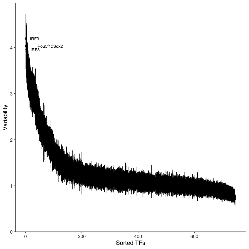
Plot variability

variability <- computeVariability(dev)

plotVariability(variability, use_plotly = FALSE)

Warning message:
“Removed 1 rows containing missing values (`geom_point()`).”

head(variability)

A data.frame: 6 × 6

	name	variability	bootstrap_lower_bound	bootstrap_upper_bound	p_value	p_value_adj
	<chr>	<dbl>	<dbl>	<dbl>	<dbl>	<dbl>
MA0004.1.Arnt	Arnt	1.3097587	1.0574367	1.539051	1.354635e-03	5.368102e-03
MA0006.1.Ahr::Arnt	Ahr::Arnt	1.6408099	1.3310370	1.897313	1.558287e-09	1.055386e-08
MA0019.1.Ddit3::Cebpa	Ddit3::Cebpa	0.9217392	0.7530152	1.071486	7.633490e-01	8.387992e-01
MA0029.1.Mecom	Mecom	1.1118984	0.9152195	1.279191	1.241110e-01	2.357689e-01
MA0030.1.FOXF2	FOXF2	1.2476069	0.9803963	1.488305	7.572098e-03	2.648457e-02
MA0031.1.FOXD1	FOXD1	1.4145492	1.1059477	1.689789	4.012849e-05	2.019982e-04

Let’s save the final results so we can compare it with pychromVAR

df_z <- as.data.frame(t(round(assays(dev)$z, 2)))
write.csv(df_z, "chromvar_z.csv")

We also save the count matrix so we can use it as input for pychromVAR

counts <- assays(example_counts)$counts
rownames(counts) <- df_peaks$peak
counts <- as.data.frame(as.matrix(counts))
write.csv(counts, "counts.csv")